
Current Version: Profex 5.2.8 - Released March 15, 2024

Introduction
Refinement presets are a simple, effective, and safe way of using a standardized refinement strategy for reoccurring sample compositions. For example in routine quality control measurements for batch release exactly the same refinement strategy should be employed each time in order to rule out operator bias.
Another advantage of refinement presets is that they reduce user input to just a few mouse clicks. This enables untrained personnel to run refinements set up by an expert without requiring to know about details of the refinement strategy.
This tutorial demonstrates how to set up and apply refinement presets in Profex.
Preparations
Download and install the latest version of the Profex-BGMN bundle.
Download example files: Examples-Presets.zip (58 kb)
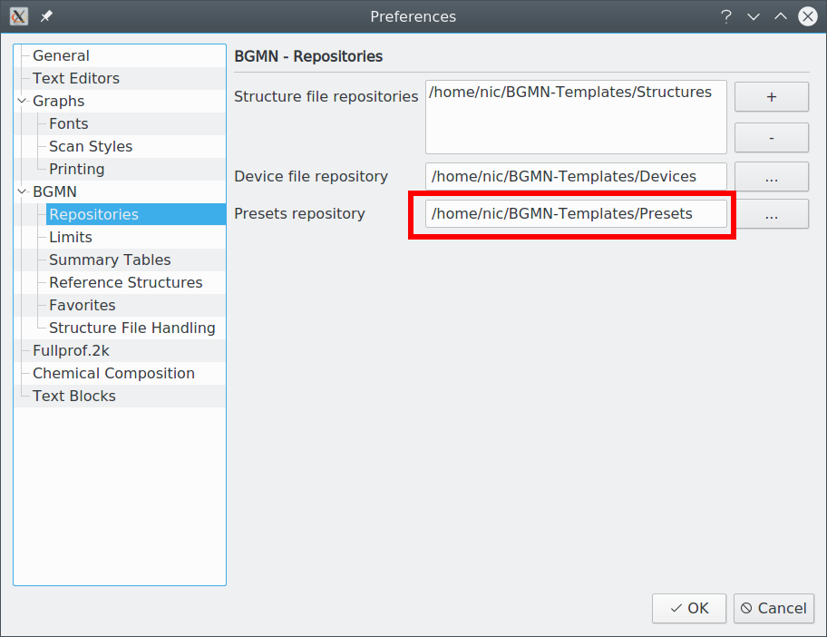
Launch Profex and go to „Edit → Preferences → BGMN → Repositories“. Check that the „Preset repository“ is a writable location. If the user creating the preset does not have write access, saving the preset will fail. In that case, change the repository to a location the creator can write to.
Creating a preset
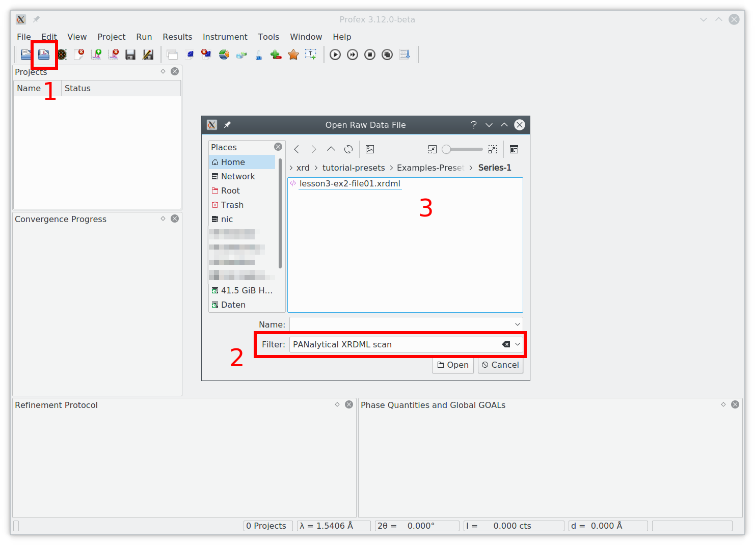
Presets are created by saving a manually optimized refinement project as a template. So we start by optimizing a refinement. Open the first file from the example files (1). Set the file format to „PANalytical XRDML scan“ (2) and select the file in the sub-directory „Series-1“ (3):
Shortcut for experienced users: Manually optimize the refinement until you are satisfied with the fit. Then proceed with saving the preset.
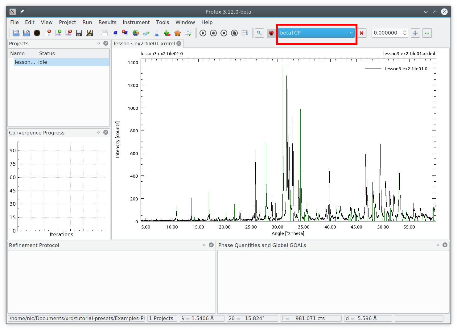
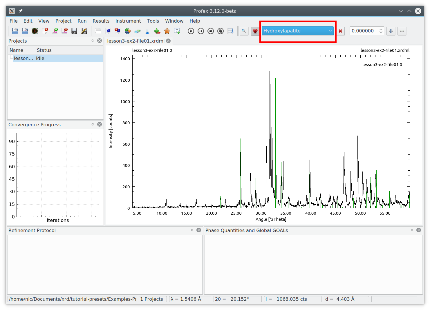
Next we need to select the phases to add by scrolling through the list of reference structures. The two phases „betaTCP“ and „Hydroxyapatite“ match perfectly
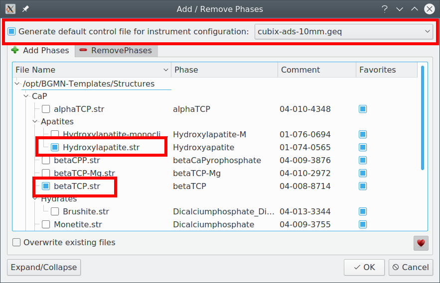
Create a project with these phases using the „Add/Remove Phase“ dialog (+– icon). Check the box „Generate default control file for instrument configuration“ and select the instrument „cubix-ads-10mm.geq“, because that is the instrument the sample was measured on. Also check the two phases „betaTCP“ and „Hydroxyapatite“. Then click OK:
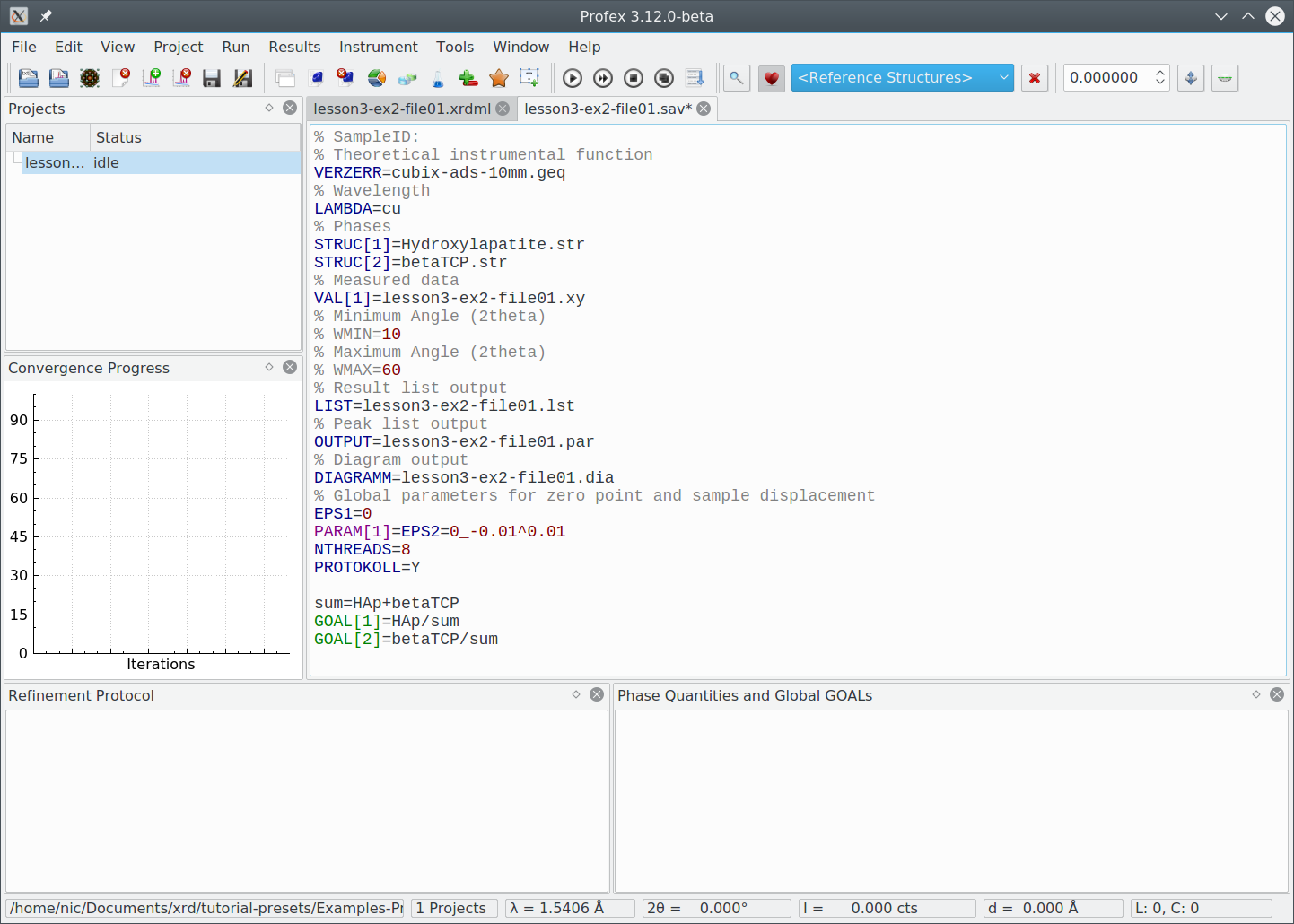
A new control file was created:
Click „Run Refinement“ to see how well the default refinement strategy works. The result looks like this:
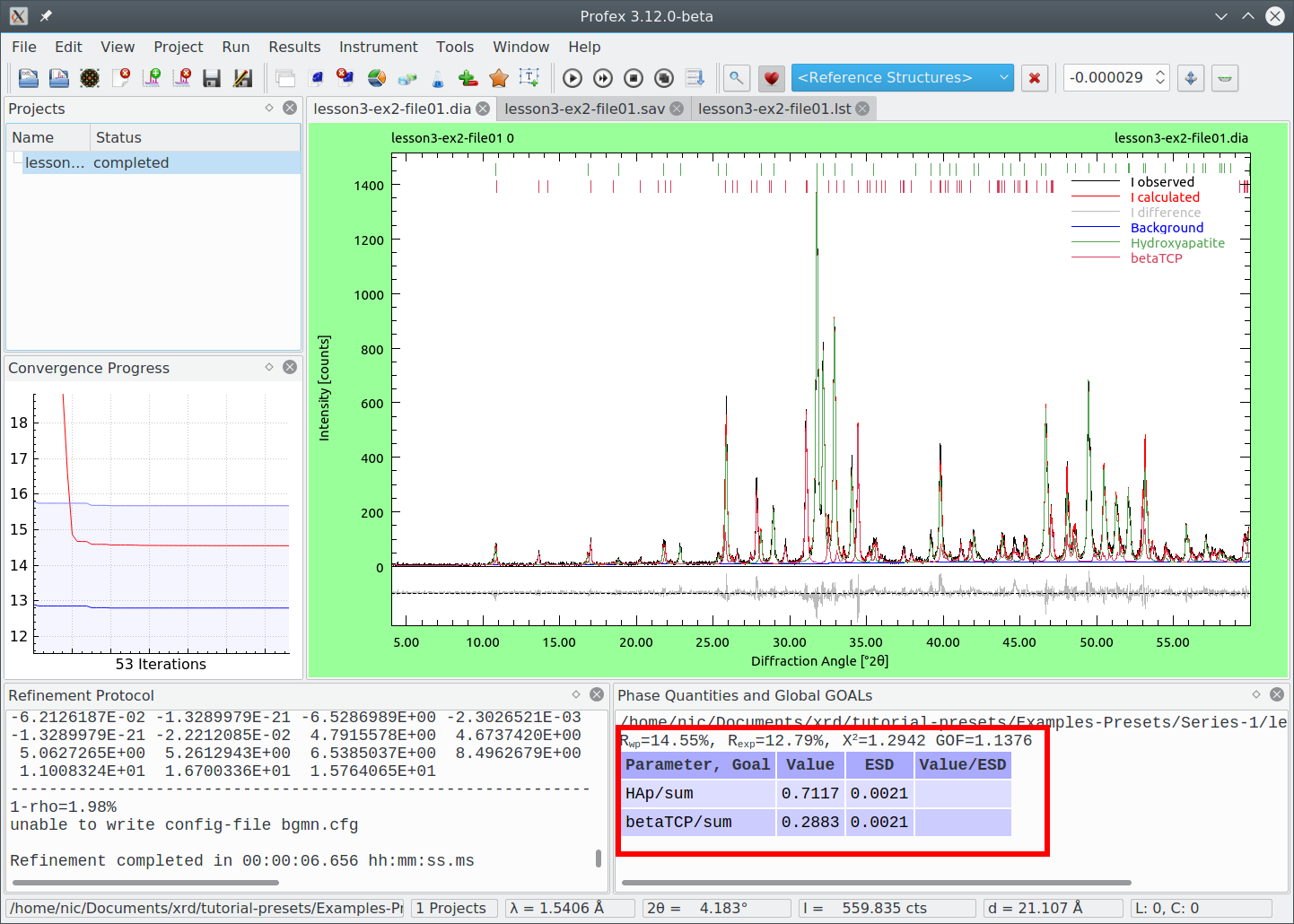
The fit looks quite acceptable. We specifically check the following:
- All peaks are assigned to either of the two phases
- The difference curve looks flat without systematic signals
- The convergence graph reached the blue area
- The goodness of fit parameters (Chi² and GOF) in the summary table are close to 1.0
However, we can still improve the refinement a bit by manually optimizing the refinement strategy. Click „Project → Open all project STR files“ to open both structure files. Apply the following changes marked red. The changes are explained at the end of this tutorial.
Control file „lesson3-ex2-file01.sav“:
% Theoretical instrumental function
VERZERR=cubix-ads-10mm.geq
% Wavelength
LAMBDA=cu
% Phases
STRUC[1]=Hydroxylapatite.str
STRUC[2]=betaTCP.str
% Measured data
VAL[1]=lesson3-ex2-file01.xy
% Result list output
LIST=lesson3-ex2-file01.lst
% Peak list output
OUTPUT=lesson3-ex2-file01.par
% Diagram output
DIAGRAMM=lesson3-ex2-file01.dia
WMIN=10
% Global parameters for zero point and sample displacement
EPS1=0
PARAM[1]=EPS2=0_-0.01^0.01
PARAM[2]=bO=1_0.2^5
NTHREADS=8
PROTOKOLL=Y
SAVE=N
sum=HAp+betaTCP
GOAL[1]=HAp/sum
GOAL[2]=betaTCP/sum
Structure file „Hydroxyapatite.str“:
PHASE=Hydroxyapatite // 01-074-0565
MineralName=Hydroxylapatite //
Formula=Ca5_(PO4)3_(OH) //
SpacegroupNo=176 HermannMauguin=P6_3/m //
PARAM=A=0.9424_0.9330^0.9518 PARAM=C=0.6879_0.6810^0.6948 //
RP=4 k1=0 PARAM=k2=0_0^0.0001 B1=ANISO^0.05 GEWICHT=SPHAR6 //
GOAL=GrainSize(0,0,1) //
GOAL=GrainSize(1,0,0) //
GOAL:HAp=GEWICHT*ifthenelse(ifdef(d),exp(my*d*3/4),1)
E=CA Wyckoff=f x=0.3333 y=0.6667 z=0.0015 TDS=0.00664290*bO
E=CA Wyckoff=h x=0.2468 y=0.9934 z=0.2500 TDS=0.00567436*bO
E=P Wyckoff=h x=0.3987 y=0.3685 z=0.2500 TDS=0.00477426*bO
E=O Wyckoff=h x=0.3284 y=0.4848 z=0.2500 TDS=0.00953535*bO
E=O Wyckoff=h x=0.5873 y=0.4651 z=0.2500 TDS=0.01014069*bO
E=O Wyckoff=i x=0.3437 y=0.2579 z=0.0702 TDS=0.01499127*bO
E=O(0.5000) Wyckoff=e x=0.0000 y=0.0000 z=0.1950 TDS=0.00000000*bO
E=H(0.5000) Wyckoff=e x=0.0000 y=0.0000 z=0.0608 TDS=0.02947459*bO
Structure file „betaTCP.str“:
PHASE=betaTCP // 04-008-8714
MineralName=Whitlockite //
Formula=Ca3_(PO4)2 //
SpacegroupNo=161 HermannMauguin=R3c //
PARAM=A=1.0439_1.0335^1.0543 PARAM=C=3.7375_3.7001^3.7749 //
RP=4 k1=0 PARAM=k2=0_0^0.0001 PARAM=B1=0_0^0.01 GEWICHT=SPHAR6 //
GOAL=GrainSize(1,1,1) //
GOAL:betaTCP=GEWICHT*ifthenelse(ifdef(d),exp(my*d*3/4),1)
E=CA Wyckoff=b x=-0.2766 y=-0.1421 z=0.1658 TDS=0.00686924*bO
E=CA Wyckoff=b x=-0.3836 y=-0.1775 z=-0.0336 TDS=0.00673765*bO
E=CA Wyckoff=b x=-0.2721 y=-0.1482 z=0.0606 TDS=0.01873909*bO
E=(CA(p),MG(0.5-p)) PARAM=p=0.5_0^0.5 Wyckoff=a x=0.0000 y=0.0000 z=-0.0850 TDS=0.01105396*bO
E=(CA(p),MG(1-p)) PARAM=p=1_0^1 Wyckoff=a x=0.0000 y=0.0000 z=-0.2658 TDS=0.01150138*bO
E=P Wyckoff=a x=0.0000 y=0.0000 z=0.0000 TDS=0.00886948*bO
E=O Wyckoff=b x=0.0070 y=-0.1366 z=-0.0136 TDS=0.02092356*bO
E=O Wyckoff=a x=0.0000 y=0.0000 z=0.0400 TDS=0.02031823*bO
E=P Wyckoff=b x=-0.3109 y=-0.1365 z=-0.1320 TDS=0.00802728*bO
E=O Wyckoff=b x=-0.2736 y=-0.0900 z=-0.0926 TDS=0.02473981*bO
E=O Wyckoff=b x=-0.2302 y=-0.2171 z=-0.1446 TDS=0.02316067*bO
E=O Wyckoff=b x=-0.2735 y=0.0053 z=-0.1523 TDS=0.00752722*bO
E=O Wyckoff=b x=-0.4777 y=-0.2392 z=-0.1378 TDS=0.01652830*bO
E=P Wyckoff=b x=-0.3465 y=-0.1537 z=-0.2333 TDS=0.00526379*bO
E=O Wyckoff=b x=-0.4031 y=-0.0489 z=-0.2211 TDS=0.01118555*bO
E=O Wyckoff=b x=-0.4246 y=-0.3056 z=-0.2152 TDS=0.01184353*bO
E=O Wyckoff=b x=-0.1814 y=-0.0805 z=-0.2233 TDS=0.01076445*bO
E=O Wyckoff=b x=-0.3696 y=-0.1748 z=-0.2735 TDS=0.01381745*bO
Repeat the refinement:
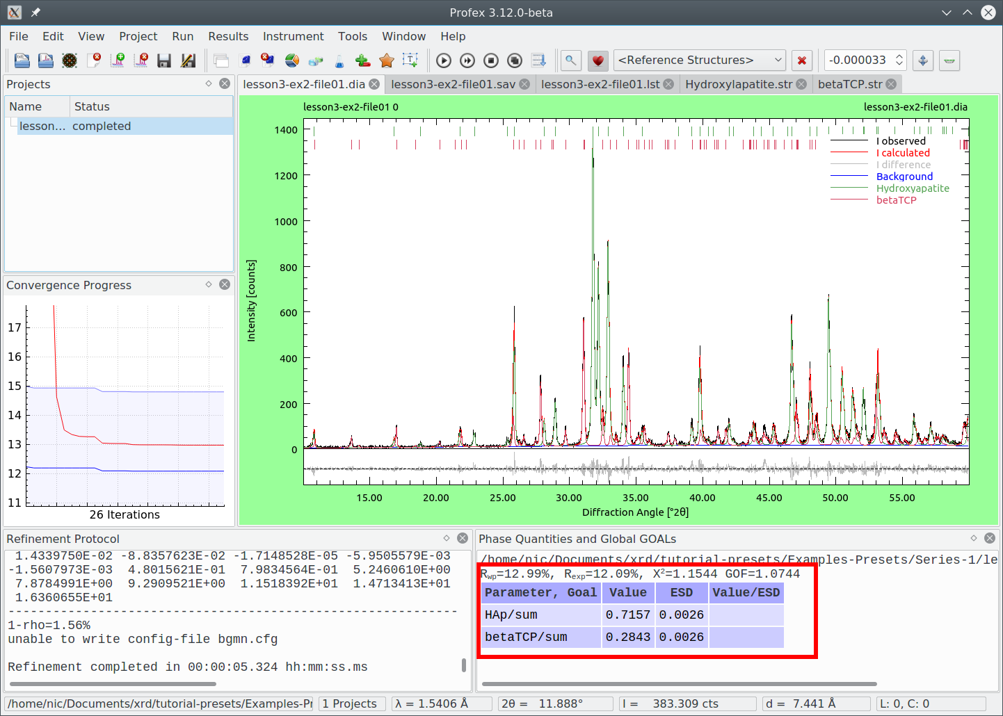
The difference curve looks a little bit flatter, and Chi² improved from 1.294 to 1.154. We are satisfied with the quality of the refinement, so we want to use the refinement strategy with the manual optimizations as our preset.
Saving the preset
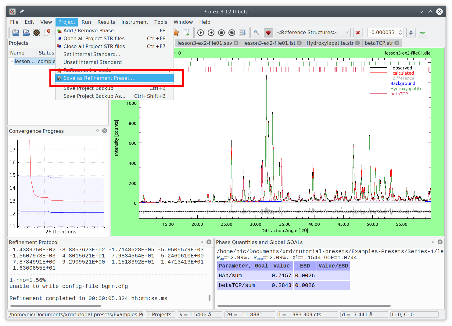
Select „Project → Save as Refinement Preset…“:
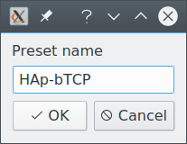
And give the preset a name, for example „HAp-bTCP“, because this is the preset that will be used to quantify bi-phasic Hydroxyapatite-betaTCP mixtures:
If the preset was saved successfully, Profex will let you know and also show the location in the refinement protocol window:
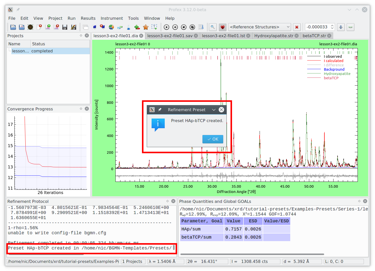
If you get an error message instead, make sure that the location where presets are stored is writable (see Preparations). The preset is ready now.
Applying a preset
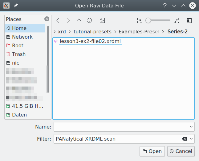
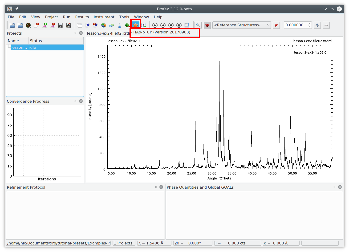
Open another scan file with similar composition. Select „File → Open raw scan file…“ and pick „lesson3-ex2-file02.xrdml“ (as shown above):
Then click the yellow star icon to open a dropdown menu showing all available presets. It will probably just contain the one we created above:
Select the preset to apply it. The same can be done by clicking the menu „Project → Refinement Presets…“. Now run the refinement by pressing the F9 key. The result looks like this:
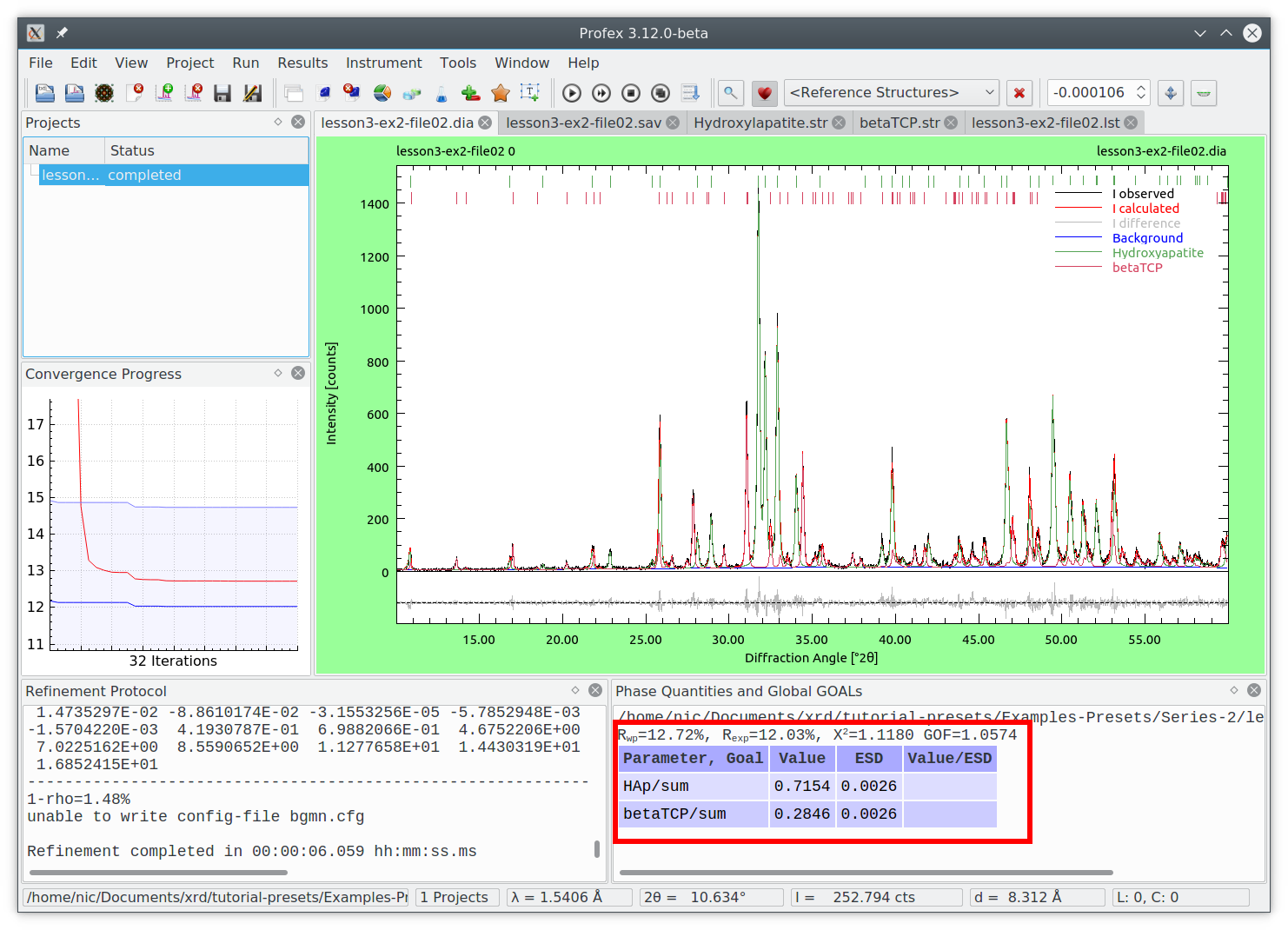
If you take a look at the structure and control files, you will notice that all the manual changes we applied above are present. Refinements from presets require no user input other than loading the file, applying the preset, running the refinement, and exporting the results.
Issues when applying presets
In some situations one or several of the following warning messages are shown when applying a preset.
Overwrite existing control file
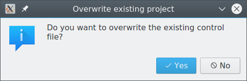
This warning is shown when a preset is applied to a project that has already been configured. Choose if you want to overwrite the control file with the version of the preset.
Checksum warning
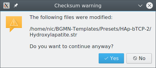
Presets are checked for (accidental or malicious) modifications when applied. If a file that is part of a preset has been modified since its creation, this warning is shown to inform the user about the inconsistency. The preset can still be applied, but the user knows about potential risks.
Overwriting existing files
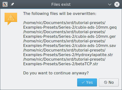
If several scan files are located in the same directory, applying a preset can lead to a conflict that would overwrite structure or instrument files copied there by another project. Sharing structure and instrument files among several refinement projects can be desired in some situations (e.g. batch refinements), but not in other cases. The user must decide whether or not overwriting the listed files causes a problem with other projects in the same directory. To avoid the conflict, abort preset application, create a new directory and move the scan file to the new directory. Then open the file from the new location and apply the preset.
Protected and shared preset repositories
In a regulated environment it may be necessary to protect the preset repository against modifications. Ideally, all users share the same repository, but only an administrator user has write-access. This can simply be achieved by setting the preset repository to a network shared drive with the desired access permissions, as described in the preparations section above. Users with read-only access will be able to use the presets, but not to modify, create or delete presets. The location will have to be changed in every new installation of Profex. Updating Profex will preserve the settings.
The preset repository can be backed up and restored, as well as moved to another location, without causing checksum warnings. Consistency checks will only verify file integrity, not the file location.
Addendum – Manual optimizations
The manual optimizations applied in section Creating a Preset above include some common strategies to improve the fit. These modifications are not directly related to presets, but they describe some common manual optimization approaches. Hence they will be explained here as further information for interested users.
Control file (*.sav)
The following keyword sets the minimum angle to 10 degrees. Data below 10 degrees will be ignored during the refinement. This was safe to do because the initial refinement showed that no peaks occur below 10 degrees. Clipping low-angle data speeds up the refinement and sometimes improves the background refinement. Do not clip ranges that contain diffraction data (peaks).
WMIN=10
A new parameter „bO“ was defined and refined between 0.2 and 5.0, starting at 1.0. This parameter was used by both structure files. Its meaning will be explained below. Parameters used by several structure files must be defined and refined in the control file.
PARAM[2]=bO=1_0.2^5
Structure file Hydroxyapatites.str
Micro-strain was released for isotropic refinement (k2) using the default limits. Texture refinement was increased from SPHAR4 (default) to SPHAR6 to refine more complex texture models.
RP=4 k1=0 PARAM=k2=0_0^0.0001 B1=ANISO^0.05 GEWICHT=SPHAR6 //
The isotropic thermal displacement parameters (TDS) of all atoms were multiplied with a refined parameter „bO“. The same value for bO is used for all atoms in both structures. This is a very robust way to refine TDS in cases where the default values are not a good choice, for example if the published data was measured at very low or very high temperature. bO is defined and refined in the control file (see above), so the same parameter can be shared by all structure files.
E=CA Wyckoff=f x=0.3333 y=0.6667 z=0.0015 TDS=0.00664290*bO
...
Structure file betaTCP.str
The same optimizations as for Hydroxyapatite.str were applied. Additionally, substitution of Mg for Ca was refined for positions Ca4 and Ca5. Site Ca4 has a site occupancy of 0.5. A parameter „p“ was defined and refined in the range from 0.5 to 0.0, starting at 0.5. It refines the ratio of Ca and Mg on Ca4.
Ca5 is fully occupied (site occupancy = 1.0) , hence the parameter „p“ can vary between 1.0 and 0.0. It describes the amount of Ca on Ca5, whereas the amount of Mg is defined as (1-p). With this model the site is always fully occupied, no vacancies are introduced, only the ratio of Ca and Mg is refined.
E=(CA(p),MG(0.5-p)) PARAM=p=0.5_0^0.5 Wyckoff=a x=0.0000 ...
E=(CA(p),MG(1-p)) PARAM=p=1_0^1 Wyckoff=a x=0.0000 ...
Nicola Döbelin, September 2017